Costs and load balancing¶

Routing decisions depend on what we choose to minimise, whether that is number of vehicles, distance, duration, or delivery load. PyVRP Enterprise supports an advanced cost model using piecewise linear functions, which can model a wide range of different cost structures for various attributes.

In this tutorial we first determine how many drivers we need by simply minimising total route duration. Once we have determined how many routes to plan, we want to balance the delivery loads across the routes. We will build a load cost using a piecewise linear function to ensure this is the case.

[1]:

import matplotlib.pyplot as plt
import numpy as np

import pyvrp
import pyvrp.stop

[2]:

data = pyvrp.read("data/belgium-n49-k10-ghent.vrp")

Minimising duration¶

We first need to determine how many drivers we need. For this initial scenario we simply minimise duration, and let PyVRP figure out a reasonable number of routes.

We only want to modify the objective, not re-write the entire data instance. To do this, we first use replace() to replace the relevant vehicle type attributes, and then again to replace the vehicle types on the data instance. In each case, replace() returns a copy of the object where the relevant attributes have been replaced by the arguments. Since we plan to use this again, we will wrap it all inside a new solve() function.

[3]:

def solve(**kwargs):
    """
    Replace vehicle type attributes with the given kwargs and solve.
    """
    vehicle_type = data.vehicle_type(0).replace(
        # Disable distance costs and set a unit duration cost.
        distance_cost=pyvrp.PiecewiseLinearFunction(slope=0),
        duration_cost=pyvrp.PiecewiseLinearFunction(slope=1),
        **kwargs,
    )

    inst = data.replace(vehicle_types=[vehicle_type])
    return pyvrp.solve(inst, pyvrp.stop.MaxRuntime(1))

[4]:

min_duration = solve()
print(min_duration)

Solution results
================
    # routes: 4
     # trips: 4
   # clients: 48
 # shipments: 0
   objective: 125547.0
    distance: 111147
    duration: 125547
# iterations: 856
    run-time: 1.00 seconds

Routes
------
Route #1: C30 C43 C33 C11 C45 C34 C35 C15 C16 C42
Route #2: C36 C1 C19 C46 C2 C5 C12 C23 C6 C20 C17 C3 C0 C27 C14
Route #3: C9 C32 C28 C41 C13 C37 C25 C18 C22 C4 C26 C10 C7 C39 C31
Route #4: C40 C29 C44 C47 C8 C38 C24 C21

PyVRP needs four drivers. Let’s see how the solution’s load is distributed across routes, using the plot_loads function:

[5]:

def plot_loads(sol, title, ax=None):
    """Plots route loads on a figure with the given title."""
    if ax is None:
        _, ax = plt.subplots()

    ranks = range(1, sol.num_routes() + 1)
    loads = [route.delivery()[0] for route in sol.routes()]
    mean_load = np.mean(loads)

    bars = ax.bar(ranks, sorted(loads, reverse=True), label="Route load")
    ax.bar_label(bars, padding=3)

    ax.axhline(
        mean_load,
        color="black",
        linestyle="--",
        label="Equal share",
    )

    ax.set_xticks(ranks)
    ax.set(xlabel="Route (#)", ylabel="Load", title=title)
    ax.legend(frameon=False)
    ax.margins(y=0.2)

[6]:

plot_loads(min_duration.best, "Scenario with duration costs")

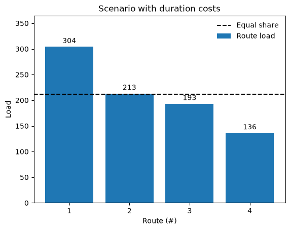
That’s not very balanced! But this was to be expected: we never told the solver that we cared about this. Let’s correct that now.

Balancing route loads¶

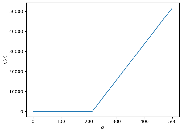
We will balance the route loads by telling PyVRP about load costs. First, we define the target: we want each route to have roughly an equal share of the total delivery load. The target load across four routes is about 212 units of load.

When a route is loaded with a load \(q\) below the target load, that does not incur additional load cost. Only when \(q > 212\) do we incur load cost: this route is overloaded, and that needs to be penalised. Using a weight term \(w\), we thus construct a function \(g(q)\) as follows:

The weight term \(w\) can be freely chosen. We use \(w = 180\), that is, we weigh one unit of overloading the same as a detour of 180 seconds.

Let’s build this function using PyVRP’s PiecewiseLinearFunction functionality, and have a look at its plot:

[7]:

W = 180
Q = data.vehicle_type(0).capacity[0]
LOAD = sum(client.delivery[0] for client in data.clients())
TARGET = LOAD // min_duration.best.num_routes() + 1

# Define a piecewise linear function between (q, g(q)) points:
# * at 0, g(0) == 0;
# * at TARGET, g(TARGET) == 0;
# * and at Q, g(Q) == W * (Q - TARGET).
points = [(0, 0), (TARGET, 0), (Q, W * (Q - TARGET))]
load_cost = pyvrp.PiecewiseLinearFunction(points)

_, ax = plt.subplots()
ax.set(xlabel="$q$", ylabel="$g(q)$")
plt.plot([load_cost(x) for x in np.arange(Q)]);

Let’s adjust the scenario and solve it again.

[8]:

num_routes = min_duration.best.num_routes()  # num drivers we need
with_load = solve(num_available=num_routes, load_cost=[load_cost])
print(with_load)

Solution results
================
    # routes: 4
     # trips: 4
   # clients: 48
 # shipments: 0
   objective: 133887.0
    distance: 118587
    duration: 132987
# iterations: 707
    run-time: 1.00 seconds

Routes
------
Route #1: C41 C13 C37 C15 C35 C34 C45 C25 C16 C42
Route #2: C40 C31 C9 C32 C7 C39 C29 C44 C47 C8 C38 C24 C21
Route #3: C36 C1 C19 C46 C2 C17 C22 C18 C4 C26 C28 C10 C27 C14
Route #4: C3 C30 C33 C11 C43 C12 C5 C23 C6 C20 C0

The objective has slightly increased, which is to be expected: we have changed the optimisation goal, so the original duration-minimal solution is no longer good. But have we achieved what we wanted to do - balance route load?

[9]:

_, (ax1, ax2) = plt.subplots(ncols=2, figsize=(9, 4.5), sharey=True)
plot_loads(min_duration.best, "Scenario with duration costs", ax1)
plot_loads(with_load.best, "Scenario with duration and load costs", ax2)
plt.tight_layout()

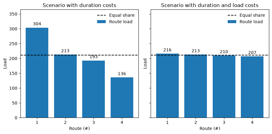
Yes we have!

Conclusion¶

In this notebook we explored various cost structures, by first minimising duration, and then designing a cost function for load that ensured balanced loads across all routes. For this we used PyVRP’s piecewise linear functions, a powerful concept for defining your own objective terms. You should now be able to use piecewise linear functions to specify your own objectives.